A Brief Intro to StyleGAN
 Kevin Zhu
What is StyleGAN?
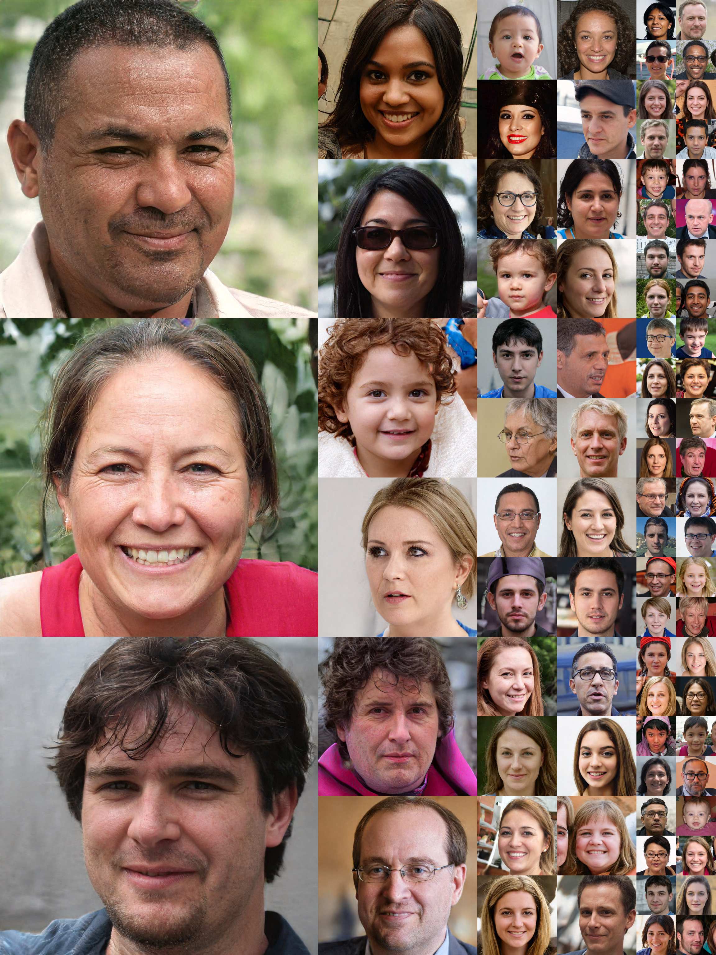
StyleGAN is a new generator architecture for GANs made by NVIDIA, that generates pixel pictures of human faces of high quality. It borrows idea from style transfer literature, and applies it to generating faces from latent codes instead. Rhe network is able to separate out details at every level, allowing independent control over global features such as pose, as well as finer details such as skin tecture and hair placement.
The network embeds the input latent code into an intermediate latent space, which is then passed into each layer of a synthesis network. The synthesis network takes in a constant tensor as input, and with the help of the intermediate latent code and some extra injected noise at each layer, it is able to progressible learn and upscale an image until we reach a human face.
Outline
In the rest of this article, we’ll cover the following:
What makes it better than previous works?
Previous networks focused alot on improving the discriminator, whereas on the generator side, they mainly worked with the distributions in input latent space to encourage certain results. StyleGAN takes a unique approach to all of this, giving it several big advantages:
- The quality of images is high, both in resolution as well as FID score.
- The intermediate latent space is learnt in such a way that it admits a more linear representation of different face attributes.
Note: I don’t have enough experience with previous works to definitively say what is better about this than prior art.
How does it work?
We start with a latent code \(\bf{z} \in \mathcal{Z}\), which is then passed through an 8 layer MLP (defined as \(f : \mathcal{Z} \to \mathcal{W}\)) to obtain \(\bf{w} \in \mathcal{W}\) in the intermediate latent space. This \(\bf{w}\) is then passed into each of the layers of a synthesis network, with a different learned affine transformation in each layer. Each of these values are called “styles”, which we can define as \(\bf{y} = (y_s, y_b)\).
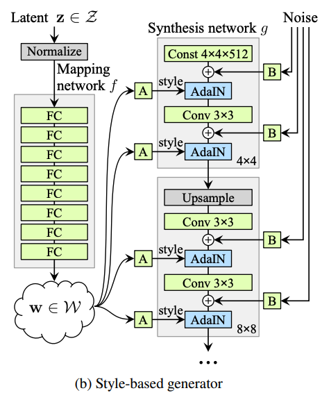
Meanwhile, we synthesis network starts off with a latent code. At each layer, we upscale the current image, inject some Gaussian noise, and then use Adaptive Instance Normalisation (AdaIN) to merge the style and image together. The formula for AdaIN is given as follows:
\[\operatorname{AdaIN}(\bf{x}_i, \bf{y}) = \bf{y}_{s, i} \frac{\bf{x}_i - \mu(\bf{x}_i)}{\sigma(\bf{x}_i)} + \bf{y_{b, i}}.\]
This has the effect of normalising each feature in the map \(\bf{x}_i\) separately, before scaling and biasing using the corresponding scalar component in style \(\bf{y}\). This continues until the final image is generated.
Cool things the paper does
Mixing together different styles
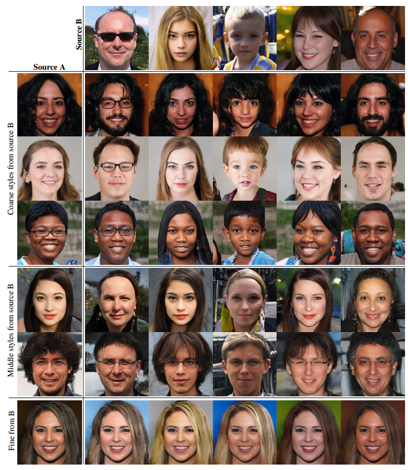
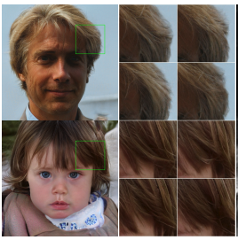
To encourage styles to localise to each layer, the authors use a technique called mixing regularisation during training. In this procedure, a percentage of images are chosen to be generated using two latent codes. It works by using one latent code up to a point, and then switching to another one. This regularisation technique helps to prevent the network from assuming adjacent styles are correlated, and thus separates out the effects of styles in each layer.
Doing this also has the great side effect that we can start mixing styles together between two completely different people. For example, we copy the coarse style from one generated image to another, we can start to see that features such as gender, age, pose and hair can be copied from one person to another.
Adding stochastic variation with noise
Typically hair tends to exhibit stochastic properties, even though the exact placement of each strand don’t matter.
In previous GANs, this would mean that the network would have to use up some of it’s bandwidth in order to generate ways to place the hair.
“Given that the only input to the network is through the input layer, the network needs to invent a way to generate spatially-varying pseudorandom numbers from earlier activations whenever they are needed. This consumes network capacity and hiding the periodicity of generated signal is difficult — and not always successful”
Hence, Gaussian noise is injected into the network at each layer in order to remove the need to generate these random numbers. Not only that, the injected noise only affects the local stochastic features, without affecting global properties such as pose or hair style. This is a known affect from previous literature
“… spatially invariant statistics (Gram matrix, channel-wise mean, variance, etc.) reliably encode the style of an image while spatially varying features encode a specific instance.”
If the network tries to control something like the pose using stochastic noise, then since the noise is by definition noisy, even close together pixels will get affected in dramatically different ways, causing a wildly incosistent poses across the iamge. This is easily picked up by the discriminiator, and thus is discouraged by the generator architecture.
Furthermore, since there is a fresh set of noise added at each layer, there is no incentive for stochastic features to use noise from previous layers. Hence, the effects of noise is effectively localised to the layer it is injected in.
Disentangling the latent space
Ideally, we would like the transformation from our latent space to the final image to be one where various final picture attributes form linear subspaces in our input latent space (e.g. one element in the input code determines the final age). This is known as disentanglement of features.
However, missing features in the training set can lead to a distorted latent space, as show in the paper. For example, consider two factors of variation (e.g. masculinity and hair length). Now assume the training data is missing one section (e.g. long haired males), as shown in (a).
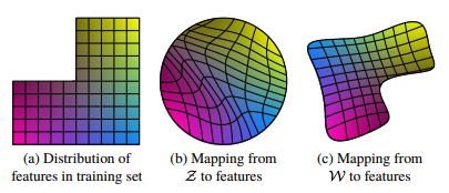
Then after a mapping from \(\mathcal{Z}\) is learned, the mapping is distorted (b) since there cannot be any gaps in the input. Therefore, the learned mapping from \(\mathcal{Z}\) to \(\mathcal{W}\) can be used to reverse the warping.
“We posit that there is pressure for the generator to do so, as it should be easier to generate realistic images based on a disentangled representation than based on an entangled representation.”
The authors describe two novel methods to measure entagnlement
- Perceptual Path Length
- A measure of how quickly an image changes as we interpolate from one point to another in \(\mathcal{Z}\)
- Linear Separability
- Label 100,000 images using a separate trained classification network based on binary attributes (e.g. gender). Then, fit a linear SVM to predict the label based on the latent-space point \(z\). The calculated conditional entropy (i.e. how surprising finding out the correct label is given the linear SVM’s prediction) roughly translates to how well the binary attribute can be described as a linear subspace.
Creating “antifaces”
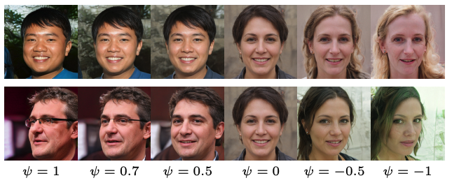
By taking the average of \(f(\bf{z})\) over the probability distribution \(P(\bf{z}))\), we can work out the intermediate latent code \(\overline{\bf{w}}\) that generates the “mean face”. It has very interesting properties, such as looking straight onto the camera, and being of an indeterminate gender.
But we can do more. For any face \(\bf{w}\), we can work out the “antiface” \(\bf{w}'\) by reflecting it around \(\overline{\bf{w}}\). This let’s us generate the opposite of each face. It’s interesting to note that various attributes such as gender, age, glasses, and looking direction all swap to their opposites in the antiface.
Updates
Since StyleGAN, there has been progressive updates to the paper. These can all be found in a blog here: stylegan.xyz/code